
Recently I have been reading Richard Feynman‘s The Feynman Lectures on Physics—trying to fill the glaring lack of pure science knowledge missing from my formal university education—and I came across his chapter on Newton’s laws of motion. He demonstrated the beauty and power of Newton’s ideas by describing how the motions of the planets can be modeled with a few simple equations. Of course his demonstration consisted of working through the equations by hand for a few time steps, but he did mention that this work could be done on the top computers of the day.
…but in modern times we have machines which do arithmetic very rapidly; a very good computing machine may take 1 microsecond, that is, a millionth of a second, to do an addition.
Given more than 40 years have passed since Feynman made that statement about 1Mhz processors, I assume I should be able to implement a model on my own modest machine. Since I am still on an astronomy kick, I could not think of a more enjoyable way to spend my time. Without further ado, let us switch to the royal we.
Planets move through our solar system in three dimensions. To model their motion through this space, we need to know their mass, position, and velocity. Mass is easy enough to find, but there appears to be a dearth of information about a planet’s (x,y,z) location in space—probably because whoever created the universe forgot to label his axes. It seems we will instead have to settle for something called ephemerides data. Given one object in space, other objects are described by angles (right ascension and declination) from the first object; a wonderful description of how to interpret those angles can be found here. This type of information is how astronomers on Earth know where to look to see other celestial bodies.
We can think of right ascension as being longitude, representing an angle east or west that is measured in hours, minutes, and seconds. Declination is then latitude, representing an angle north or south that is measure in degrees. First we will describe where to get the data and then we will deal with translating it to an (x,y,z) location.
Obtaining the Ephemerides Data
Not surprisingly, NASA is the place to ask for data like this. They provide a web interface to their HORIZONS system for generating the data. We just need to select a few options. Our most important choice is Observer Location; we want a common center point for every object in our system. The ideas of Copernicus seem pretty solid at this point, so choosing the Sun to be our center—our (0,0,0) if you will—is a logical choice. To be blatantly Earth-centric, we will choose Earth for our first Target Body. The final choice is the date and time, which should obviously be the same for every body we wish to model. We will begin with the not so random data of February 9th, 1986 at midnight. Our reasons for this choice will be clear in Part 2.
Once the data is generated, only the information from a few of the columns are needed. The ascension data is in columns 3, 4, and 5; the declination data is in columns 6, 7, and 8. The final piece of information is the column labeled delta. Given in terms of astronomical units (AU)—one AU is 149,597,870.691 kilometers, the average distance from the Earth to the Sun—delta is the distance between the two objects. Not only will we collect the data from midnight, but also 1:00am, one hour later. Given the position of the planet at two points in time, velocity information can also be estimated.
Converting the Data to Coordinates
Before converting the ephemerides data to spatial coordinates, we should also decide on the scale of our axes. For simplicity, we will use an AU scale for each axis. Given the information we already have, we can easily calculate coordinates in the (x,y,z) space with high school geometry. First step is to convert the unfamiliar hours and degree units to radians—recall that radians are an angle measurement between 0 and 

Declination is instead measured by degrees, minutes, and seconds. Here minutes are just a subunit of a degree; each degree is subdivided into 60 minutes. We can convert declination to radians in a similar manner.

Now that we have a proper angle measurement, the rest of the data is obtained by the simple geometry of a right triangle. It is easiest to begin with the z coordinate. The hypotenuse is the distance between the Sun and the object of interest. The coordinate z is the height of the triangle. For the moment, we will label the base of the triangle A. The angle we just calculated, 
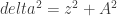

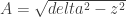
Using a little algebra, we can solve for z.

Calculating x and y requires knowing A, which can be calculated by
In order to calculate x and y, we rotate the space and consider a new right triangle. The hypotenuse is now A, x is the base, and y is the height. The angle 


We can repeat this process for an additional point to calculate the velocity in each direction.

Checking our Work
A couple of tests, while not proof the above math is correct, are suggestive that we are on the right path. Using the (x,y,z) coordinates, the distance from the Sun to any other object can be recalculated. This value should match the original delta value from NASA’s data. From the velocity values, we can also calculate the overall speed of the Earth. From our calculations, we obtain about 109,000 km/h. Wikipedia sets the Earth’s orbital speed at 107,000 km/h, reasonably close to our answer. Finally, if we repeat the calculation on the Moon, the distance between the Earth and Moon should be around 380,000 km. Our calculations give 377,000 km, also very close.
Next Step
It took a bit of effort, but we can now plot any object in our solar system in an (x,y,z) space. In Part 2, we will set the planets in motion. I also promise to provide some basic C++ code to both convert the ephemerides data to (x,y,z) points and to model their motion throughout space. Please let me know if anything is unclear or incorrect.

Pingback: Modeling the Solar System, Part 2: Setting the Planets in Motion | William Hartmann